As humans, we have an innate and natural tendency to establish patterns and associations in our environment. Consider for a moment, the capability of the human brain to “process millions of visual, acoustic, olfactory, tactile, and motor data, and…the astonishing ability to learn from experience, generalize from learned rules, recognize patterns, and make decisions”. The ability to recognize patterns allows us to distinguish objects one from another; to interpret sound waves as speech; and to understand the unique patterns of individual letters that collate to form words and sentences.
These skills provide meaning, knowledge, and experience to the observer. It is difficult to mimic this type of pattern recognition and establishment of data relationships in a computational context.
In other words, how do you train a computer to evaluate disparate datasets in order to recognize the difference between desert and forest conditions or understand the type of complex relationships that the human mind can resolve after many years of experience?
As datasets increase in number, size, dimensionality, and complexity, there is also an increase in the need to develop a computationally-based pattern recognition classification system that provides a consistent mechanism for reducing complex observational and derived datasets (e.g., multi-spectral sensors; in situ measurements, land use, terrain metrics, patch densities, etc.) into more meaningful forms that enhance our decision making processes.
Pattern Recognition and Classification Spatial and temporal processes have an explicit cause-and-effect relationship to the landscape and spatial patterns. Through the collection of data by means of observation (i.e., field-collected, instrument collected, remotely-sensed, etc.) or
data derivation, patterns in and between these data can be extracted to better understand the biotic or abiotic factors that have the power to influence ecological relationships, hydrological functions, or other natural or anthropogenic system processes.
Once the relationships in these patterns are established, pattern recognition technologies can be used to predict and define data or provide new insights to a study area.
The implementation of pattern recognition can be applied to a “landscape” such that a spatial perspective can be gained. A landscape is fundamentally composed of a patchwork of potentially recognizable spatial units, that could vary in extent and character depending on the variables used to identify homogeneous areas.
The fuzzy nature of process and function boundaries and the multiple scales at which these boundaries are observed increases the complexity of landscape classification. In addition, it can be difficult to recognize hidden and/or unknown process interactions through observation alone.
It is also important to consider that, the concept of landscape is not limited to natural elements, but may also include anthropogenic systems operating over any spatial domain (e.g., transportation systems, demographics, renewable energy production, agricultural efficiency, etc.).
The notion of landscape classification and the determination of homogeneous areas continue to be an important research area for many disciplines including geography, ecology, hydrology, water resource management, land-use planning, and environmental management. The

multi-disciplinary need for regionalizing the landscape, or dividing it into simpler domains, resulted in a wide variety of classification methods ranging from direct observation and interpretation to more objective statistical approaches, including maximum likelihood classifier, k-means, linear and quadratic discriminate analysis, decision trees, multivariate regression, and Bayesian networks;
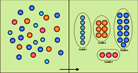
However each of these methods have known limitations when dealing with complex, non-linear, non-Gaussian distributed data. Regardless of the classification theme (e.g., landscape units, species distribution, demographics, etc.), the objective of classification is to reduce complexity and facilitate the interpretation of the real world by grouping similar elements together to provide a convenient abstraction from the original observations (see Figure 1). Classification of data is critical to promoting clear and effective decision making.
Artificial Neural Networks Artificial Neural Networks (ANNs) can be used to develop a classification procedure which blends traditional statistical methods with a machine learning approach, allowing the system to iterate over a collection of datasets until patterns can be learned and realized.
This concept introduces the notion of “adaptive learning” and is especially effective for evaluating data that continually evolves in time and space, such as meteorology, vehicle traffic, the spread of disease, and landscape processes. The use of ANNs in landscape classification have been researched and developed, however, they are not as commonly used as the statistical methods discussed previously.
It is possible the limited used of ANNs in landscape classification are due to the overall complexity of the process, the many different types of ANN models available, and the notion that these are “black box models”. Some authors refer to ANNs as “universal approximators of any multivariate function…of particular interest for modeling highly nonlinear, unknown, or partially known complex systems, plants, or processes.” ANNs are considered semi-parametric classifiers because they use both parametric discriminate functions and non-parametric shape discriminators.
While ANNs have their foundations in conventional statistical models, they differ in that;
1) Gaussian, or normal, distributions of data are not required;
2) linear or nonlinear data are acceptable for inputs;
3) adaptive learning is an integral part of the model; and
4) there is a high degree of error tolerance, provided a reasonable signal-to-noise ratio exists in the data. ANN models make no assumptions about the input data and allow for an automatic determination of parameters (i.e. adaptive learning) through the evaluation and repeated weighting adjustment of the input data space.
As stated by Perus and Krajinc, “the most important thing is that ANNs allow for a different view of problems which cannot be solved by [exact] statistical methods due to their theoretical limitations.”
The Self-Organizing Map The Self-Organizing Map (SOM) is an unsupervised ANN that projects and maps high-dimensional, complex, linear, or nonlinear data into iteratively organized clusters in a topology-preserving geometric structure for the creation of a low-dimensional discrete data space.
This technique is used for a wide variety of purposes, including speech recognition, industrial process control, image analysis, data mining, anomaly detection, DNA sequencing, data visualization, climate downscaling, demographics, and more.
The SOM “…can be characterized as a two-dimensional, finite-element ‘elastic surface’ or network that is fitted to the distribution of the input samples,” says Kohonen.
The added value of the SOM is its ability to discover hidden data patterns, structures, and relationships in multivariate datasets.
It can also conceptualize and map data in one-dimensional (1-D), two-dimensional (2-D), or three-dimensional (3-D) output space using a variety of topological structures (e.g., linear, rectangular, toroidal, spherical, cubic).
Because the SOM classifies data in an unsupervised form, no training data are presented to the network; thus, no a priori knowledge about the data distributions or placement of data into discrete output space is incorporated.
The SOM structure (see Figure 2) is obtained by interatively presenting the same input data signals to the network and adjusting the network weights to create “meaningful order, as if some feature coordinate system were defined over the network” (see Figure 3) (Kohonen, 2001).
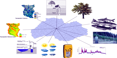
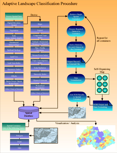
“Scientists at the U.S. Department of Energy’s Pacific Northwest National Laboratory (PNNL), developed a GIS/ANN-based application, referred to as the Adaptive Landscape Classification Procedure (ALCP). ”
The ALCP was specifically developed to: 1) address the classification of large, complex geoinformation datasets; 2) overcome the limitations of traditional classifiers; and 3) blend the unique and complementing power of GIS and ANNs.
The ALCP combines the advanced geospatial information extraction, data storage, and analysis capabilities of a GIS and a particular type of ANN, called the Self-Organizing Map (SOM), to provide a topology-preserving means for reducing and understanding complex data relationships across a given landscape (see Figure 4).
Varying types and forms of data, including vector data (i.e., lines, points, and polygons), raster, thematic, spatiotemporal, continuous, discrete, and multi-scale data can be assimilated in the ALCP to address different management needs such as hydrologic response, erosion potential, habitat structure, climate zones, physiographic regions, hazard/risk analysis, feature identification, instrumentation placement, monitoring design, forecasting, what-if scenarios, and more.
The ALCP uses neurocomputing-based pattern recognition to provide a unique insight to spatial and spatiotemporal phenomena.
There are three specific objectives that the ALCP works to accomplish.
First, establish data relationships and structure among large, complex, linear or non-linear, high-dimensional datasets.
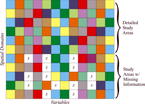
For example, an evaluation of spatial data signatures (see Figure 5) extracted from a common spatial domain across many datasets and data derivatives reveals complex patterns that can be grouped according to similarities in their data signal.
Second, the ALCP provides an approach for inferring landscape processes in areas that have limited data available but exhibit similar landscape characteristics as other areas with a more detailed and complete set of observations.

Data relationships can be derived from data-rich spatial domains for the purpose of filling-in missing data in other spatial domains that tend to share similar characteristics (see Figure 6).
Lastly, the ALCP can help measure the sensitivity of individual variables or groups of variables that influence landscape processes and response.
This can reveal variables in the landscape that are primary process drivers for a range of conditions and scenarios (e.g., what variables have the greatest influence over water availability in the summer vs. winter? Also consider high elevation vs. low elevation, high relief vs. low relief, high latitude vs. low latitude, etc.).
The ALCP uses the notion of a “spatial container” to: 1) define the region(s) of interest for analysis; and 2) capture, organize, and normalize the data that falls within the bounds of a container (see Figure 7).
The spatial container itself is a collection of features comprised of one or more, contiguous or non-contiguous points, lines, or polygons, located within the study area.
For example, a spatial container may be defined by one or more vegetation boundaries, land use types, catchment boundaries, population densities, monitoring locations, migratory routes, traffic routes, or other representative features.
Once defined, the spatial extents of the features in the spatial container are used to extract any intersecting source layers, which may vary by scale and data type, into a unified structure stored in a spatial database.
It is important that, collectively, the features within all the spatial containers provide sufficient variability among their attributes, enabling the ACLP to derive meaningful spatial patterns and data relationships. This concept is no different than the requirement for deriving typical statistical metrics.
The ALCP is undergoing continuous development and is still considered a research tool; however, its strength, evolution, and adaptability as a tool, comes through its application to real-world problem-sets. Several of these applications are briefly presented to give a sense of the types of problems that can be addressed.
Multi-Spectral Imagery Classification Early applications of ALCP tested its ability to classify multi-spectral imagery into seven land class types without a priori knowledge.
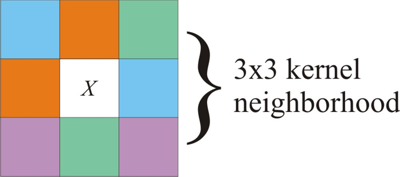
Results were then compared to ground truth data. The test used all four spectral bands on the Landsat TM and each of 9 values in a 3×3 kernel window that ultimately, was used to predict the land type in the center of the kernel window (see Figure 8).
Each data pattern presented to the ALCP consisted of an ID# for each pixel and 36 values (4 spectral bands x 9 values in the kernel window). The land classes were ground-truthed for each of the 6,435 pixels in the dataset; however, this was a blind test and these values were only used for comparison after the classification was complete.
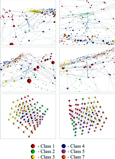
A confusion matrix (see Table 1) revealed an average agreement of 86% with the ground-truth data. Figure 9 reveals the input data space and natural and structured SOM mesh that was projected onto the data.
Table 1. A confusion matrix showing classified and misclassified data by class. Values indicated by bold-italic typeface indicate correctly classified values. All data are presented as percentages.
|
|
1 |
2 |
3 |
4 |
5 |
7 |
|
1 |
96.19 |
0.29 |
1.09 |
0.00 |
2.07 |
0.00 |
|
2 |
0.00 |
95.85 |
0.00 |
0.46 |
2.81 |
0.39 |
|
3 |
1.42 |
0.57 |
86.68 |
6.02 |
0.15 |
1.95 |
|
4 |
0.06 |
1.00 |
9.11 |
69.21 |
2.22 |
10.29 |
|
5 |
2.33 |
2.15 |
0.27 |
0.46 |
83.70 |
3.58 |
|
7 |
0.00 |
0.14 |
2.86 |
23.84 |
9.04 |
83.78 |
Table 1 – A confusion matrix showing classified and misclassified data by class. Values indicated by bold-italic typeface indicate correctly classified values. All data are presented as percentages.
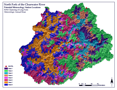
The bottom two figures display the final projected SOM in structured space. Using spatially distributed 30-year mean monthly climate data, the ALCP was used to determine the best locations for the placement of additional meteorology stations to supplement three existing stations.
The proposed stations are essential for improving knowledge of current watershed conditions, thus leading to better forecasting and decision making capabilities related to water supply, water quality, flood events, environmental constraints, and hydropower operations.
A total of 3,075 spatial containers were developed based on sub-catchment boundaries derived from 10-m digital elevation models.
At first observance of the ALCP classified data (see Figure 10), it was apparent that the underlying topography in the watershed was dominating the trend in the classifications.
Keep in mind, the ALCP had no knowledge of the topographic structure or elevation in the watershed, only the mean monthly meteorological data was presented.
Additional analysis revealed that minimum temperature and precipitation were the most sensitive to the effects of topography.
It also became clear that other meteorological variables didn’t have a strong correlation to elevation, thus using a simple elevation band or elevation band/aspect classification approach to locate a meteorology station would not be effective.
To finalize the analysis, areas were calculated for each of the classes and it was determined that 53% of the watershed was already represented by the three existing meteorology stations, with each station falling into their own unique class (classes 2, 6, and 8 in Figure 10).
If a fourth station were placed within class 7, the next largest class in terms of area, the represented area would increase by an additional 17% providing meteorological monitoring for 70% of the watershed.
If additional resources were available in the future, this same analysis could be used to determine the fifth best station placement, and so on. This application of the ALCP allows for the efficient planning of available resources and ensures proper instrument placement for monitoring ground conditions.
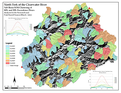
Watershed Characterization
A more complex analysis was conducted with the ALCP in an effort to understand the hydrologic properties of sub-catchments in an area with limited ground data. This type of analysis allows for efficient field data collection and monitoring since the collected data can be propagated across the catchment to other areas that exhibit similar properties.
Multivariate regression analysis conducted by the United States Geological Survey (USGS), used to determine hydrological properties of ungaged catchments, was compared with classification results from the ALCP. A total of 160 sub-catchments were tested, revealing an 82% agreement between the two methods (see Figure 11).
An additional 12% of the basins were out of agreement by one class boundary. While there are specific and defensible reasons for the differences (i.e., differences in underlying data used for each analysis), the ALCP accomplished the task in a few days versus the multi-year effort for the USGS to develop and test the regression equations.
Additionally, the use of multivariate regressions must be evaluated carefully as these types of statistical methods are not adaptable and rely solely on past observations. With shifts in climate patterns and a higher frequency of extreme events, relying upon historical observation alone will increase the level of uncertainty for understanding data relationships, determining classification boundaries, and understanding future conditions.
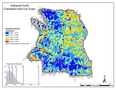
Determination of Erosion Potential
An ongoing project involves using the ALCP to determine the potential for soil erosion using spatially-derived variables, including: 1) remotely-sensed canopy and ground cover; and 2) various terrain model derived metrics that represent processes affecting rates of erosion on the landscape.
These types of analyses can target restoration efforts and/or reveal areas that should be considered carefully before implementing land use change policies.
A total of 4,478 spatial containers were derived using 1st-order catchment boundaries covering a 1,458 km2 area.
The resulting data (see Figure 12) from a multi-year project to develop a mass and energy balance hydrology and erosion model (DHSVM-HEM) is being used to compare ALCP results (Wigmosta, et al., 2008).
Provided the results of this analysis are comparable, the ALCP may prove to be a more efficient alternative for determining erosion potential in the landscape; however, it is important to keep in mind that without any known rates of erosion in the landscape, the ALCP cannot make a specific assessment of sediment loads, but rather, only determine where differences exist.
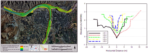
Determination of HydroGeomorphic Stream Reaches
An experimental study is being conducted to determine whether the patterns of river cross-sections, upstream and downstream thalweg elevations, and channel slope can be presented to the ALCP in order to determine hydrogeomorphic stream reaches (see Figure 13).
This type of classification is important for a wide variety of reasons, but ultimately provides a means to segment a stream or a river by its physical, and subsequently, biological processes.
Most commonly, the determination of a stream reach is developed by direct observation and delineation, and while there are guidelines to follow in this process, it is ultimately a subjective process.
The application of the ALCP in this regard proposes to offer an objective method for determining stream reach boundaries and allow a simplified approach to increase or decrease the number of stream reaches depending on the level of detail required.
Detection and Prediction of Salmon Spawning Beds
Multiple environmental criteria including, river bed material, water depth, and water velocities, affect the location of salmon spawning beds. Each year Fall Chinook salmon leave the ocean and return to their native freshwater rearing grounds to spawn.
Because these species of salmon are listed as a Threatened and Endangered Species in the United States, monitoring the health and populations are required to help understand the stressors.
One method of monitoring the populations is to locate and map the spawning beds which are only visible through the water for approximately 3-weeks during spawning period.
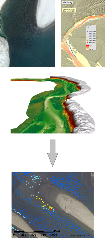
The current approach for collecting this data is to: 1) conduct aerial surveys of the spawning beds and do visual counts and rough mapping of the areas, and 2) collect aerial imagery and manually digitize the spawning beds.
An ongoing study is using the ALCP with a number of supporting datasets, including true color aerial imagery, channel bathymetry , and modeled water velocities, water surface elevations, and water depth, to automatically capture the location and extent of the spawning beds (see Figure 14).
In addition, the data relationships developed through this process can be used to predict the location of other likely spawning areas.
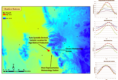
Determination of the Most Suitable Meteorology Station Data for Biofuels Model Input
The demand for developing sustainable renewable energies has brought algae-based biofuels back into the active research domain after nearly two-decades of limited research and development. To understand the potential for setting up large-scale, open-air, algae ponds throughout the United States, a nationwide, multi-criteria,
GIS-based suitability analysis is being conducted. The areas determined suitable for algae production are then run through a full mass and energy balance hydrodynamic algae pond model developed at the Pacific Northwest National Laboratory. The primary intent of the algae pond model is determine the required water usage and potential production rates under varying climates and water chemistries. One of the primary inputs to the algae pond model is meteorology data, as the weather parameters are highly-influential to pond water temperature, evaporation rates, and productivity rates.
Using the ALCP, data relationships are being built between a spatially-distributed, mean monthly climate dataset (containing multiple parameters such as maximum/minimum temperature, precipitation, dew point, etc.) and meteorology station data. The objective of this research is to select the most representative meteorology station within a defined proximity to the GIS-determined suitable area (see Figure 15).
In many cases the selected meteorology station will turn out to be the closest station to the suitability-determined area, however there is enough variability through topography and existence of microclimates, that the nearest feature method will not capture the most representative station.
The ALCP provides a powerful and adaptive procedure capable of processing large volumes of complex data, discovering relationships and patterns in the data, and reducing the data complexity to a more meaningful form by classifying common data patterns.
The developed procedures can be used to propagate detailed information learned from a given spatial domain to other areas in the landscape without the same level of detailed information.
This notion, among other things, allows for the intelligent and efficient pre-planning of research and monitoring studies to effectively capture the unique aspects in the landscape, and then apply the learned information to the “data gaps” or areas in between the specific study sites.
The procedure is well suited for use in adaptive environmental modeling, research, monitoring, and management, as well as a predictive capability for a wide range of topic areas (i.e., determine probable locations of groundwater recharge zones, ideal restoration and/or protection areas, field sampling and instrument location sites, land use assessment, risk assessment, forecasting, data filling, and “what-if” scenarios for various impacts, etc.) and is specifically intended to be adaptive in the types of data that can be used and the problem sets it can be applied to (i.e., not necessarily limited to addressing landscape-based questions).
With the dramatic increase in the amount of available spatial information over the past three-decades, as well as the huge advances made in the GISciences, it is necessary to implement more modern approaches to handling and resolving data such that we can effectively use all of the information that is available to us to maximize decision making opportunities.
————————————————————————————————
André Coleman is a senior research scientist at the Pacific Northwest National Laboratory in Richland, Washington, USA. Mr. Coleman specializes in the Geographic Information Sciences (GISc) as applied to hydrologic modeling, evolutionary computing/machine learning technologies for pattern recognition, classification, and data optimization, distributed computing, advanced terrain analysis, and real-time data harvesting for near real-time modeling.
He was enrolled at UNIGIS – Free University of Amsterdam, where he was the winner of the Academic Excellence Prize 2008 based on his high quality MSc thesis at the GI_Forum 2009 in Salzburg, Austria. His dissertation entitled: “An Adaptive Landscape Classification Procedure Using Geoinformatics and Artificial Neural Networks” was considered unanimously by the Review Board as the best thesis this year. Email, [email protected]; Web: http://www.pnl.gov
References
Bação, F, V Lobo and M Painho. (2004), Geo-self-organizing map (Geo-SOM) for building and exploring homogeneous regions, Geographic Information Science, Proceedings. Lecture Notes in Computer Science, pp. 22-37.
Bação, F., V. Lobo, and M. Painho (2008), Applications of Different Self-Organizing Map Variants to Geographical Information Science Problems. In: P. Agarwal and A. Skupin (eds.), Self-Organising Maps – Applications in Geographic Information Science. John Wiley & Sons, Ltd., West Sussex.
Bailey, R.G. (2004), Identifying ecoregion boundaries. Environmental Management, 34 (Suppl 1):S14-S26.
Bathgate, J.D. and L.A. Durham (2003), A geographic information systems based landscape classification model to enhance soil survey: A southern Illinois case study. Journal of Soil and Water Conservation, 58(3):119-127.
Bryan, B.A. (2006), Synergistic techniques for better understanding and classifying the environmental structure of landscapes. Environmental Management, 37(1):126-140.
Chon, T.S., Y.S. Park, K.H. Moon, and E.Y. Cha (1996), Patternizing communities by using an artificial neural network. Ecological Modelling, 90(1):69-78.
Ehsani, A.H. (2007), Artificial Neural Networks: Application in Morphometric and Landscape Features Analysis, KTH, Royal Institute of Technology, Stockholm, pp. 53.
Hewitson, B.C. (2008), Climate Analysis, Modelling, and Regional Downscaling Using Self-Organizing Maps. In: P. Agarwal and A. Skupin (eds.), Self-Organising Maps – Applications in Geographic Information Science. John Wiley & Sons, Ltd., West Sussex.
Hilbert, D.W. and B. Ostendorf (2001), The utility of artificial neural networks for modelling the distribution of vegetation in past, present and future climates. Ecological Modelling, 146(1-3):311-327.
Hsieh, B.B. and M.R. Jourdan (2006), Watershed Similarity Analysis for Military Applications Using Supervised-Unsupervised Artificial Neural Networks. In Proceedings of the 25th Army Science Conference, Orlando, Florida.
Joy, M.K. and R.G. Death (2004), Predictive modelling and spatial mapping of freshwater fish and decapod assemblages using GIS and neural networks. Freshwater Biology, 49(8):1036-1052.
Kecman, V. (2001), Learning and Soft Computing. MIT Press, Cambridge, Massachusetts, pp. 541.
Kohonen, T. (1982), Self-organized formation of topologically correct feature maps. Biological Cybernetics, 43(1):59-69.
Kohonen, T. (2001), Self-Organizing Maps. Springer-Verlag, Berlin, Germany, pp. 501.
Lenz, R. and D. Peters (2006), From data to decisions – Steps to an application-oriented landscape research. Ecological Indicators, 6(1):250-263.
Openshaw, S. and C. Openshaw (1997), Artificial Intelligence in Geography. John Wiley & Sons, Ltd., Chichester.
Park, Y.S., I.S. Kwak, T.S. Chon, J.K. Kim and S.E. Jorgensen (2001), Implementation of artificial neural networks in patterning and prediction of exergy in response to temporal dynamics of benthic macroinvertebrate communities in streams. Ecological Modelling, 146(1-3):143-157.
Perus, I. and A. Krajinc (1996), AiNet: A Neural Network Application for 32-bit Windows Environment (Version 1.25), User’s Manual. Celje, Solvenia. Accessed February 6, 2007 at
http://www.winsite.com/bin/Info?500000014622 (undated webpage).
Schmuker, M., F. Schwarte, A. Brück, E. Proschak, Y. Tanrikulu, A. Givehchi, K. Scheiffele, G. Schneider (2007), SOMMER: Self-Organizing Maps for Education and Research. Journal of Molecular Modeling, 13(1):225-228.
Turner, M.G. (1989), Landscape ecology: the effect of pattern on process. Annual Review of Ecological Systems, 20:171-87.
Wigmosta, M.S., L.J. Lane, J. Tagestad, and A.M. Coleman (2009), Hydrologic and Erosion Models to Assess Land Use and Management Practices Affecting Soil Erosion, ASCE J. of Hydrological Engineering, (14) 1, p. 27-41.
