 The reduction of land maintenance actions has determined a need for awareness about soil conservation issues. The main consequence is an increasing soil loss due to flash flood or similar phenomena. This issue needs a new approach leading to a continuous analysis and monitoring action. This part’s aim is to describe the main steps of the development of the GIS-based methodology to assess soil stability through GIS modelling. Specifically, soil physical structure has been studied by evaluating its aggregate stability. In order to follow a multidisciplinary approach data obtained from the laboratory analysis has been merged with topographical information and vegetation cover records.
Turin Hillside Case study: soil vulnerability
The second study area includes nine towns close to Turin (Piemonte, NW Italy). It ranges from 200 m m.s.l. to 670 m m.s.l. with an extension of near 7000 hectares (45° 6′ 6″N; 7° 45′ 56″E).
In order to focus on soil, 82 samples (0–15 cm topsoil) located in the whole area have been collected; representing the vegetation cover typologies of the area as described in the regional forest inventory and available in shapefile format in the Region website. These information have been employed in order to plan the sampling location with the purpose of assuring the representativeness of the survey.
WAS (Wet Aggregate Stability) index have then been applied on soil samples in order to assess the soil aggregate stability, i.e. the stability of aggregates in the 1-2 mm diameter range. The aggregate loss was determined after different wet sieving times (5, 10, 15, 20 40 and 60 minutes) using a rotating sieve apparatus (Yoder, 1936; Pojasok, 1990; Dickson et al. 1991).
The model improved by Zanini et al. (1998) has been adopted, describing aggregate failure with a kinetical approach. Aggregate losses at fixed times are fitted to an exponential model through an iterative procedure:
y(x) = b+a(1-e-x/c) (1)
Where:
y = aggregate loss
t= time of wet sieving
b= failure of aggregates for explosion at water saturation
a= maximum estimated abrasion loss
c= parameter linking the rate of breakdown to the abrasion time.
The rate of aggregation breakdown is described by the first derivative:
y'(x) = (a/c)e-x/c (2)
As a, b and c, taken individually, are only the expression of a single feature with physical meaning (explosion, abrasion and time of total breakdown), they can not describe the global behaviour of disaggregation processes. In order to reduce the kinetic variability to a single parameter and compare the stability of different vegetation covers, a scalar approach can be carried on. Miller (1980) and Simmons et al. (1979) developed a scaling method applied to aggregate breakdown curves, obtaining a scale mean curve Y*(t) such as that each time series Yi (t), estimated from measured yi(t) values, can be represented as a linear function of Y*(t) according to the following relation:
λrYi (t) = Y*(t) (3)
where the scale mean time series Y*(t) were derived from
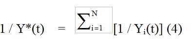
where N is the number of time series.
The scale factor values λr were obtained by minimizing the squared misfit
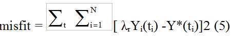
subject to the constraint 1/N  λr = 1. The scale mean curve was computed from the 82 time series using (3) and the scale factors λri derived from a forward Newton iteration using (5).
In order to obtain a spatial information from the sampling points the λr values has been interpolated by using an IDW algorithm (Tomeczak M., 2003), generating a raster used in the next phases of the research (Figure 2, on the left).
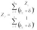
Where:
Zj = unknown value
Zi = measured point
β = weighing power
δ = smoothing parameter
hij = Euclidean distance between the interpolated node j and the contributing data point i.
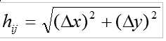
Where:
Δx = horizontal distance
Δy = vertical distance
Since soil vulnerability is also affected by geomorphology, the digital terrain model (DTM) of the study area have been computed in raster format with a 25m grid, in order to include this factor in the analysis. Then the LS (Slope-length) factor, which appears in the USLE-RUSLE Equations, describing the effect of topography on soil water erosion, has been calculated, by applying the equation developed by Mitasova et al (1996):
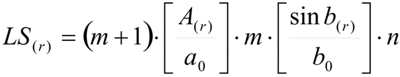
Where:
A[r] = upslope contributing area per unit contour width
b = slope
m, n = empirical parameters
a0 = 22,1 m. i.e. USLE standard plot length
b0 = 9%, i.e. USLE standard plot slope
The final result is another raster layer represented in Figure 1 (on the right).
Then every raster computed has been reclassified using a five classes subdivision according to project methodology.
In alternative to empirical approaches such as the USLE-RUSLE methods (Wischmeier and Smith, 1965, 1978) a function based on measured vulnerability data synthesized by the λr parameter have been adopted:

Vulnerability = f(λr;LS) (9)
The function has been developed b aggregating the two rasters using map algebra, and the final result has been classified according to the same criteria as presented in Figure 1.
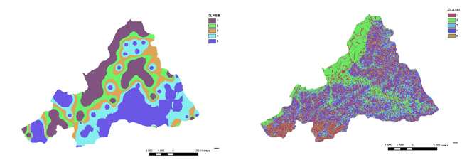
Figure 1. IDW map of λr parameter (equation 6) and LS factor raster layer (equation 8)
Results
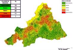
The vulnerability map (Figure 2) shows the hazard levels with the extension of each class. The “Low” and “Medium” classes prevail in terms of area percentage. The medium class is almost completely represented by flat areas, while scarce vegetation cover plays a role in soil stability affecting the distribution of higher vulnerability values (Zanini et al., 1998). On the other side area affected by high hazard level are located on steep slopes. Since the function includes both vegetation cover and geomorphology, areas with similar topography can show different behaviour, namely a different susceptibility to erosion.
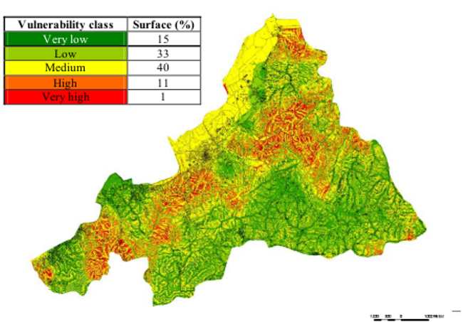
Figure 2. Vulnerability map
Project Application
The described experimental phases have led to the application of the project in the whole Turin Province. Planning, management and field competences have been delegated to “Comunità Montane”, i.e. group of associated municipalities in mountain or hillside areas. Each is responsible for planning and applying maintenance actions on its territory, on watershed basis.
As shown in the next figure, computed from data published in Province’s report (Rossi, 2007) up to the 65% of the basin have their planning phase fulfilled (Figures 3).
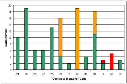
Figure 3. Summary of the planning phase in each “Comunità Montana” (green: completed; orange: work in progress; red: missing)
The following executive phase has been activated in, approximately the 46% of the areas (Figure 4).
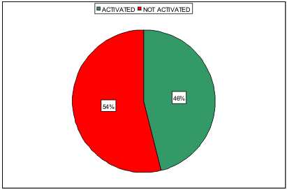
Figure 4. Percentage of “Comunità Montane” which have activated the executive phase
Conclusions
The final results succeeded both in the aim of statistical and cartographical accuracy, providing a synthetic tool for land planners not skilled in GIS or soil science. Maps are not supposed to describe punctual erosion phenomena, but they allows technicians to point out areas prone to different level of soil vulnerability, in order to plan specific land maintenance strategy and to carry on management actions. Currently the project has been adopted by the regional government, thus extending its application to the whole territory.
Acknowledgements
This work is a part of a Strategic Programme involving the Province of Turin and the Corintea (Society of independent professionals), supervised by the. Faculty of Agriculture. The base maps were obtained from Regione Piemonte Cartographic Service and IPLA Spa.
———————————————————————————-
D. Godone¹; G. Garnero¹; R. Chiabrando¹; A. Caimi²; S. Stanchi²; E. Zanini²
¹Turin University – DEIAFA, Via Leonardo da Vinci 44, 10095 Grugliasco (TO) Italy – [email protected]
² Turin University – DIVAPRA, Via Leonardo da Vinci 44, 10095 Grugliasco (TO) Italy
References
ARPA Piemonte, 1999. Rapporto sullo stato dell’ambiente Torino, ARPA.
Chiabrando, R., Garnero, G., Godone, D., Caimi, A., Stanchi, S., Zanini, E., 2004. A guide-line for territorial maintenance: development of a GIS-based method. In GISRUK Conference Proceedings. Norwich (UK), pp. 360-364.
Dickson, J.B., Rasiah, V., Groenvelt, P.H., 1991. Comparison of four prewetting techniques in wet aggregate stability determination. Can. J. Soil Sci., 71, pp 799-801.
Hippoliti G., 1994. Le utilizzazioni forestali Firenze, CUSL.
Lorito S., Vianello G., Stanchi S., Zanini E., 2003, A 3D approach to evaluate natural hazard and risk assessment in the Alpine Ecosystem : the case study of a winter sport area (Part 1- Part 2). GISRUK 2003 Proceedings. London, City University. pp. 308-312.
Mitasova, H., Brown, W.M., 2002. Using Soil Erosion Modelling for Improved Conservation Planning: A GIS-based Tutorial Geographic Modelling Systems Lab. University of Illinois at Urbana-Champaign.
Pojasok, T., Kay, B.D, 1990. Assessment of a combination of wet sieving and turbidimetry to characterize the structural stability of moist aggregates. Can. J. Soil Sci. 41, pp. 67-72.
Rossi, C. (Editor), (2007), La Manutenzione Ordinaria del Territorio nella Provincia di Torino – I Dati della Fase Attuativa, Provincia di Torino. 15 pp.
Tomeczak, M., 2003. Spatial interpolation and its uncertainty using automated anisotropic inverse distance weighing (IDW)–Cross-validation/jacknife approach. In Mapping radioactivity in environment – Spatial Interpolation Comparison, 97. G. Dubois, J. Malczewski, M. de Court (Eds.) European Commission – Joint Research Centre, pp. 51-62.
Wischmeier, W.H., Smith, D.D., 1965. Predicting rainfall erosion losses from cropland east of the Rocky Mountains. Agr. Research Serv. Agriculture Hand-book 282, USDA, Washington.
Wischmeier, W.H., Smith, D.D., 1978. Predicting rainfall erosion losses. A guide to conservation planning. USDA, Washington.
Yoder, R. E., 1936. A direct method of aggregate analysis and a study of the physical nature of soil erosion losses. Agron. J. 28, pp. 237-351.
Zanini, E., Bonifacio, E., Albertson, J.D., Nielsen, D.R., 1998. Topsoil aggregate breakdown under water saturated conditions. Soil Sci, 163, pp. 288-298.
Website:
Regione Piemonte Forest Inventory Webpage:
http://www.regione.piemonte.it/montagna/foreste/pianifor/info.htm
